These macros have been developed at the Applied Superconductivity Center to help in the quantification of microstructural features that are important to the properties of superconducting wires and cables and to make representation of those results in figures and presentations more helpful to readers. They have been made available here as a contribution to the development of these techniques in the superconductor community and to demonstrate the power of the ImageJ macro language. Disclaimer (of course): We assume no responsibility whatsoever for its use by other parties, and make no guarantees, expressed or implied, about its quality, reliability, or any other characteristic. On the other hand we hope you do have fun with them without causing too much harm.
The applications of some of these macros are described in more detail in:
Sanabria C, Lee PJ (2022) "An Introduction to Digital Image Analysis of Superconductors. Handbook of Superconductivity", Chapter G1.4:46–70, in the Handbook of Superconducting Materials - 2nd Edition, Ed. in Chief, D. A. Cardwell and D. C. Larbalestier, pub. Taylor and Francis, Abingdon, UK. ISBN-13: 78-1439817322
![]() The GitHub repository is here: https://github.com/peterjlee
The GitHub repository is here: https://github.com/peterjlee![]()
![]() ImageJ/Fiji: There is an extensive official ImageJ repository of example macros at this link, and even more can be found at the ImageJ wiki site at this link. The ImageJ community is also very supportive and requests made to the members via the ImageJ mailing list and forum can be a good source of information.
ImageJ/Fiji: There is an extensive official ImageJ repository of example macros at this link, and even more can be found at the ImageJ wiki site at this link. The ImageJ community is also very supportive and requests made to the members via the ImageJ mailing list and forum can be a good source of information.
Macro Collections:
Minimum (and Maximum) Distance MeasurementsMany microstructural features change in size, distribution, morphology and chemistry with distance from an interface (i.e. relative to a diffusion source or a diffusion barrier). This macro adds the minimum distance between the centroid of a set of analyzed objects and a reference set of points to the ImageJ results table. This data can then used to provide position normalized quantification of microstructures, microchemistry and even images as in this publication: DOI:10.1017/S1431927600037624
A reference location file with X coordinates in column 1 and Y coordinates in column 2 is required (using standard mageJ delimeters - e.g. a tab separated txt file exported by ImageJ or a csv file).
The macro can use imported XY values that are in pixels or to the same scale as the active image
but if the active image is calibrated the macro will generate both pixel and scaled information.
The latest version can be found here: link
Up to 20 additional columns (12 optional) are added to the Results table in the current version:
Minimum distances to the reference set (and the coordinates of the minimum location).
The added columns can be relabeled with a global prefix and/or suffix.
Maximum distances to the reference set (and the coordinates of the maximum location).
Minimum distances to the center (based on mean of coordinates) of the reference set.
Angle of minimum distance direction (degrees).
Angular offset of minimum distance angle from Feret angle.
If the image is scaled, additional columns of "unscaled" pixel values will be added.
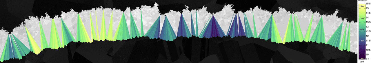
The minimum and maximum distance lines can be drawn as overlays. LUTs can be used to color code the lines according to any parameters in the Results table.
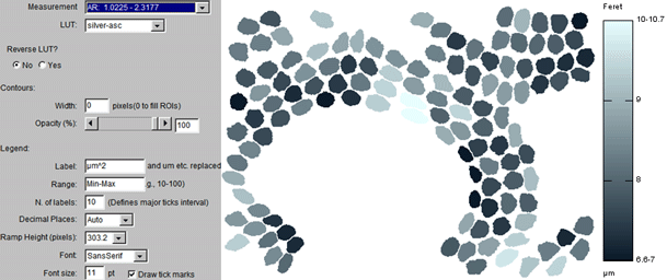
The BAR ("Broadly Applicable Routines") collection maintained by Tiago Ferreira has numerous features worth exploring and one of our favorites is the ROI color coder annotation macro that allows you to color each analyzed object with a color based on any set of feature values. We have extended the formatting options of this macro to provide more flexibility; the number of options might look intimidating but the defaults should be reasonable choices and scale with image size. If you would like to try these variants out they are available in this: directory. To cite the original BAR scripts (issued under the GNU General Public License (GPL)) use: https://doi.org/10.5281/zenodo.495245
5 Variants:
BAR ROI Color-Coder + auto-prefs: Additional features include:
1. The measured range of values is shown for all measurements in the Measurement selector (this makes it easier to manually select a range for the color ramp).
2. The selected LUT (color lookup table) can be reversed.
3. Default values are calculated for the legend range and intervals so that the intervals are typically integers.
4. An automatic suggested value for the decimal places can be selected (based on the magnitude and range of the values).
5. A ramp height is suggested base on the image height.
6. Parameter and unit labels added to the top an bottom of ramp respectively.
7. Overrun labels are added to the ramp if the true range exceeds the range chosen for the ramp (see example below).
This is useful when there are just a few outliers that would otherwise reduce the contrast variation for the majority of the features.
8. Any previous ramp is closed before creation of a new ramp.
9. Provides an option at the end to create a new merged image combining labeled image and legend (the legend/ramp height is scaled to match the height of the image).
The GitHub location is: https://github.com/...
BAR ROI Color-Coder with ROI-Manager Labels:
Additional features over the autoprefs macro listed above:
Each ROI is renamed with the chosen feature value and these are used as labels.
BAR ROI Color Coder with Scaled-Labels:
Additional features over the autoprefs macro listed above:
Each ROI is labeled with the chosen feature value using extensive formatting options. If Gabriel Landini's "Morphology" plugin is installed it will allow you to center the labels at the morphological centers of the objects (better than centroids for complex shapes because these points are always inside the original objects).
BAR ROI Color Coder + ScaledLabels + Summary: As above but now also has a Summary table option. The example below shows the histogram on the right and ≥ 3 sigma outliers outlined in red.
Line Color
We have also adapted the BAR annotator to color lines too and this is how the animated banner at the top of this page was created (as well as the example below). The latest version of this variant can be found in this: directory.
Return to Macro Collections menu
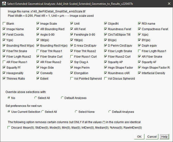
It is easy to extend the geometrical analyses provided in the standard ImageJ Analyze Particles analysis as the most common geometrical descriptions can be calculated from this basic data set. To demonstrate this we add historically common descriptions such as area equivalent diameter and fiber thickness to the ImageJ Results table using the macro in this: directory.
Some additional measurements in this version are:
Interfacial density (assuming each interface is shared by two objects - e.g. grain boundary density).
Area equivalent diameter (AKA Heywood diameter): The "diameter" of an object obtained from the area assuming a circular geometry.
Perimeter equivalent diameter: The "diameter" calculated from the perimeter assuming a circular geometry.
Spherical equivalent diameter: The "diameter" calculated from the volume of a sphere (Russ page 182) but using the mean projected Feret diameters to calculate the volume.
Roundnesss_cAR: Circularity corrected by aspect ratio, from Y. Takashimizu and M. Iiyoshi, "New parameter of roundness R: circularity corrected by aspect ratio," Progress in Earth and Planetary Science, vol. 3, no. 1, p. 2, Jan. 2016. DOI: 10.1186/s40645-015-0078-x
Round end ribbon thickness ("snake") from repeating half-annulus (Lee & Jablonski LTSW'94).
Two calculated fiber widths obtained from the fiber length from John C. Russ, Computer Assisted Microscopy, page 189.
Fiber length from fiber width (Lee and Jablonski LTSW'94; modified from the formula in John C. Russ, Image Processing Handbook 7th Ed. Page 612).
Two estimates of fiber length and two examples of volumetric estimates from projections obtained from the formulae in John C. Russ, Computer Assisted Microscopy page, 189.
Additional shape factors: "Compactness" (using Feret diameter as maximum diameter), "Convexity" (using the calculated elliptical fit to obtain a convex perimeter), "Thinnes ratio", "Extent ratio", Curl etc.
"CircToEllipse Tilt": Angle that a circle would have to be tilted to match measured ellipse (180/Π) * acos(1/AR).
Square geometries appropriate to HV (hardness) indents:
Sqr_Diag_A = √(2*Area) for a NSEW square this length should match the bounding box height and width
Like circularity the following "squarity" values should approach 1 for a perfect square:
Squarity_AP = 1-|1-(16*Area)/Perimeter2| (perhaps too sensitive to perimeter error)
Squarity_AF = 1-|1-Feret/(A*√2)|
Squarity_Ff = 1-|1-√2/Feret_AR|
Hexagonal geometries more appropriate to close-packed structures than ellipses:
HexSide = √((2*Area)/(3*√3))
HexPerimeter = 6 * HexSide
Hexagonal Shape Factor "HSF" = abs(P²/Area-13.856): Hexagonal Shape Factor from Behndig et al. and Collin and Grabsch (1982)
Hexagonal Shape Factor Ratio "HSFR" = abs(13.856/(P²/Area)): as above but expressed as a ratio like circularity, with 1 being an ideal hexagon.
HexPerimeter = 6 * HexSide
Hexagonality = 6 * HexSide/Perimeter
Full Feret coordinate listing using new Roi.getFeretPoints macro function added in ImageJ 1.52m.
Preferences are automatically saved and retrieved from the IJ_prefs file so that favorite geometries can be retained. Help button provides more information on each measurement.
Return to Macro Collections menu
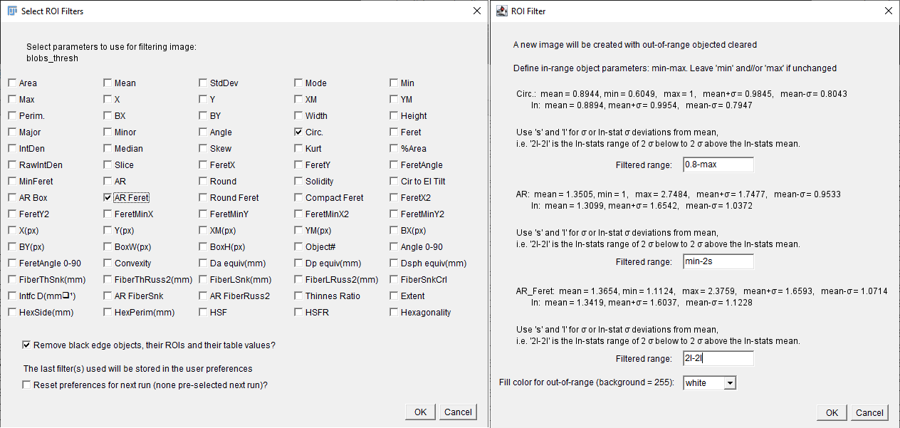
Filter ROIs by any table values
The standard ImageJ/Fiji analyze options makes it easy to filter by object area and circularity and the Biovoxxel Extended Particle Analyzer extends this filter capability to 14 standard parameters but what if you want more? This macro allows you to filter ROIs by any parameter in the Results table. This makes it possible to filter using the extended geometrical features above or for feature values created by other plugins, for instance the Particles4 and Particles8 plugins included in the "Morphological Operators for ImageJ" set developed by Gabriel Landini.
Additional features include:
Preferences are automatically saved in the ImageJ user preferences file.
The mean and standard deviations (including ln-based values) are displayed for each chosen parameter.
Standard deviation based ranges can be easily selected.
The filtered-out object color can be changed.
Create a Grid of ROIs from a Single Selection
Creates a rectangular grid of ROIs that are identical to the current selection.
The original purpose was to create ROIs for scanned 35 mm film strips.
Create Overlays of the Same Style for each ROI
Forces all overlays to have the same style.
Create Transparent Overlay_for_Selected ROI
Creates a transparent overlay from the selected ROI.
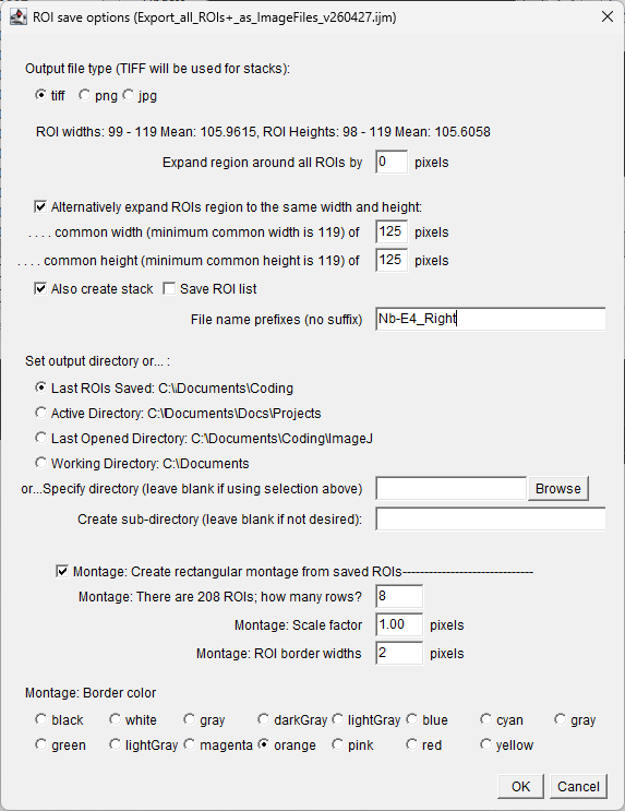
Export All ROIs as Individual Image Files
Exports all ROIs as individual image files. An expanded region our the ROIs can also be included for context and the region size can be set to the same values for all ROIs-clips. You can also create a stack and montage the ROI images. The menu below shows the current options.
Export all ROIs in a Selected Area
Exports a collection of ROIs based on the selected area.
Set ROI Color and Transparency
Opens up a dialog similar to the built-in ROI properties dialog but adding drop-downs for fill and stroke color selection and sliders for transparency.

Sort ROI Set by Proximity to Current ROI Set
Sorts an archived ROI set by proximity to the current ROI set.
Sort ROIs to a Rectangular Grid
The original order of objects (and ROIs) is by a top-to-bottom, left-to-right scan and if you have x,y grid of analysis points this may not exactly match the intuitive column/row order you would expect. You can use this macro to sort the ROIs of a rectangular grid into column-by-column, row-by-row order. This is particularly useful when combining with the export ROIs as image files macro above so that montaging the ROIs back into the same grid pattern respects the original arrangement. This macro was created to handle grids of microhardness indents.
Requirement: The rows must not overlap with each other and ROIs are already in the top-left:bottom-right order that would be expected from Analyze Particles.
- Sorts ROIs
- Adds row and column numbers to ROI name
- Appends original ROI name to final ROI name for reference
- Option to add ROI names to re-measured Results Table

Return to Macro Collections menu
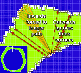
These macros (link) measure the minimum wall thickness of open or closed objects from the perspective of each pixel on the interior or exterior of a wall. If the wall is broken (incomplete) there is a version that uses an interior object to define the open and closed regions (this also allows a measurement of the percent of wall that is open). A detailed explanation of the two macros is provided in this presentation: PDF. In the illustration below we illustrate the impact of the choice of direction for this macro.
These macros (link):
1: Count the number of objects that are touching each other.
2: Count the number of objects within successive separation range increases of 1 pixel up to 10 pixels.
3: Add the minimum separation distances to the Results Table.
By default it is assumed that all objects have been previously separated by using a watershed tool (i.e. "touching" objects will be separated by 1 pixel). However, you can choose if the watershed adjustment is applied. Pixel separations are converted to the scaled unit if there is one (if just pixels are preferred just remove the scale prior to running the macro). The CZS version applies scale information from the header of CZS format TIFF headers.
Return to Macro Collections menu
This macro measures the closest separation between neighboring objects. The minimum spacings are added to the Results table along with the connecting coordinates. The spacing connecting lines can be displayed on the images or animated. Alternatives the lines can be color coded by the Line Color Coder macro using the coordinates generated with this macro.
Distances are measured from outline to inline so that objects separated by one pixel should yield a separation of 1 pixel (outline-outline would produce overlapping outlines).
Return to Macro Collections menu
Two macros (link) to add morphological centroids to the Results table based on the "MCentroids.txt" example macro by Gabriel Landini: Link. These macros require Gabriel Landini's "Morphology" plugin. These centroids are obtained by thinning objects (assuming white objects) and thus are always within object boundaries, making them useful for labeling objects. The Morphological Centroids can also be generated on request by our object labeling macros if the Morphology plugin is available.
A set of very simple macros: (link) for automating the task of saving the pixel coordinates of all non-background pixels in multiple images.
Return to Macro Collections menu
These label macros use outlines and shadows to create labels on images that stand out against the image underneath.
Legal Notice:Fancy Scale Bar
This macro (link) adds extensive formatting options to the original version by Wayne Rasband that was subsequently enhanced by Frank Sprenger. The scale bar can be an overlay or applied to the original or a copy of the image. If the image is in color there are multiple color options (the selection is restricted to grayscale choices for grayscale images to retain the original bit depth). The units can be changed from the original embedded scale (i.e. from nm to µm etc.).
The scale bar can also be placed under the image (on the right or left sides):
Using the line selection tool the precise length and angle can be shown (single or multiple arrows can be used):
If a line selection tool is used the text can be rotated to the measured angle and arbitray text can be used for the label.
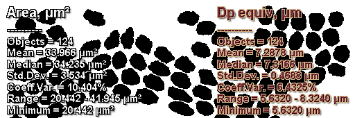
Fancy Summary Label Table
This macro (link) adds up to 8 lines of statistical summary to an image. There are extensive formatting options including outlines and shadows to help the text stand out against the image. If the image is in color there are multiple color options.
Fancy Text Labels
This macro (link) adds up to 8 lines of user created text to an image. There are extensive formatting options including outlines and shadows to help the text stand out against the image. If the image is in color there are multiple color options.
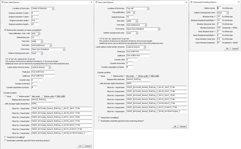
Fancy Slice Labels
This macro (link) adds multiple lines of text to a copy of the image. Sequential numbers can be added as well as prefixes and suffixes. Text in the slice labels can be globally replaced. Non-formated slice labels can be applied with more counter variables and previews to images using ImageJ's "Label Stacks" and Dan White's (MPI-CBG) "Series Labeler", so you might want to try that more sophisticated programming first to see if it meets your needs sufficiently. You can also try utilize imageJ's "stack sorter."
Magneto optical images by Anatolii Polyanskii.
Fancy Feature Labeler
This macro (link) adds scaled result labels to each ROI object.
Fancy Feature Labeler with Summary
This macro (link) adds scaled result labels to each ROI object and a summary of selected statistics.
Fancy Border
This macro (link) adds a color border to a selection. The border can consist of up to 3 layers of different thickness and can be a non-destructive overlay.
Return to Macro Collections menu
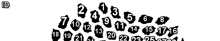
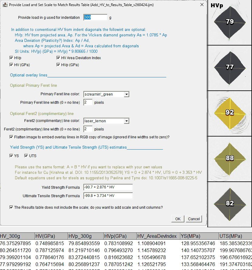
Measure hardness from diamond hardness indents and add to Results table
This ImageJ macro:
1: Uses Feret axes to measure the Vickers Hardness values from diamond indents taken with known loads and adds them to an open Results table.
2: Optionally uses projected area to measure the Vickers Hardness values from diamond indents taken with known loads and adds them to an open Results table.
2: Optionally estimates the Yield Strength and Ultimate Tensile strength from the HV values.
3: Optionally draws the Feret axes on the selected image.
Requirements
This macro requires that the indents have been thresholded and Analyze Particles has already been run with the indents added to the ROI manager.
Return to Macro Collections menu
Olympus DSX Utilities (not available for PRECiV software)
The default image format used by the original software for Olympus DSX microscopes is a two layer TIFF, which makes it very easy to use the images in ImageJ/Fiji. Unfortunately the newer PRECiV software does not support saving of individual frames montage frames so it is not possble to use these macros. The TIFF header very usefully contains complete metadata on the image acquisition parameters.
Simple ImageJ/Fiji macros that make it easier to stitch image mosaics generated by Olympus DSX microscopes.
The following macros can be down loaded from this GitHub repository.
For very large images, the DSX software only export scaled down version of assembled mosaics, so it is useful to have alternative ways of stitching very large images.
Two versions of this macro are provided:
IJStitch_DSX_Mosaic_From_Selected_Image(new_plugin)
IJStitch_DSX_Mosaic_From_Selected_Image(old_plugin)
They correspond to the 2 available versions (*new* and *old*) of the Fiji stitching plugin by Preibisch et al.: Please note that the Stitching plugins available through Fiji, are based on a publication:
Preibisch, S., Saalfeld, S., & Tomancak, P. (2009). Globally optimal stitching of tiled 3D microscopic image acquisitions. Bioinformatics, 25(11), 1463–1465. doi:10.1093/bioinformatics/btp184
and the authors request citation if they are used successfully.A third macro:
MIST-Stitch_DSX_Helper
uses the MIST plugin available from NIST to perform the tile alignment and stitching:
T. Blattner et al. "A Hybrid CPU-GPU System for Stitching of Large Scale Optical Microscopy Images", 2014 International Conference on Parallel Processing, 2014 doi: 10.1109/ICPP.2014.9
J. Chalfoun, et al. "MIST: Accurate and Scalable Microscopy Image Stitching Tool with Stage Modeling and Error Minimization". Scientific Reports. 2017;7:4988. doi: 10.1038/s41598-017-04567-yThese macros use default parameters that work well with typical images acquired at the Applied Superconductivity Center, but you will probable need to play around with them to optimize the stitching for other types of images.
Stitch height-map from registered stitching coordinates
The Stitch_height-map_from_registered_stitch_coords macro can use the tile coordinates generated above to fuse the corresponding height maps.
The macro requires that ImageMagick is installed in the system and will look for the most likely locations.
For MIST global-positions files, the dsx images need to be in the same directory.DSX batch image and height map extraction macro
Convert_Active_DSX_Image_And_All_Others_in_Same_Directory_and_Extract_HMaps
As the name implies, uses the file location of an opened DSX image to convert all the other images and extract height maps. Partially based on code by Alex Herbert and by Michael Schmid-3 and structured after the ImageJ BatchProcessFolders example macro
For height map extraction, the macro requires that ImageMagick is installed in the system and will look for the most likely locations.Olympus DSX Image Annotator
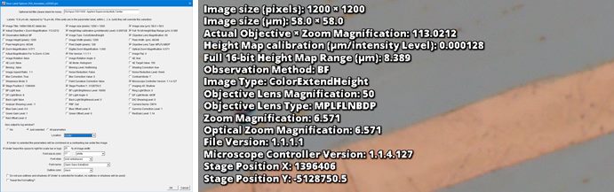
A simple ImageJ macro (link) that extracts the metadata from the header of an Olympus DSX digital microscope image and creates a formatted label of selected paramters on or below the image. It also sets the image scale if it has not been previously set.
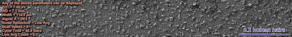
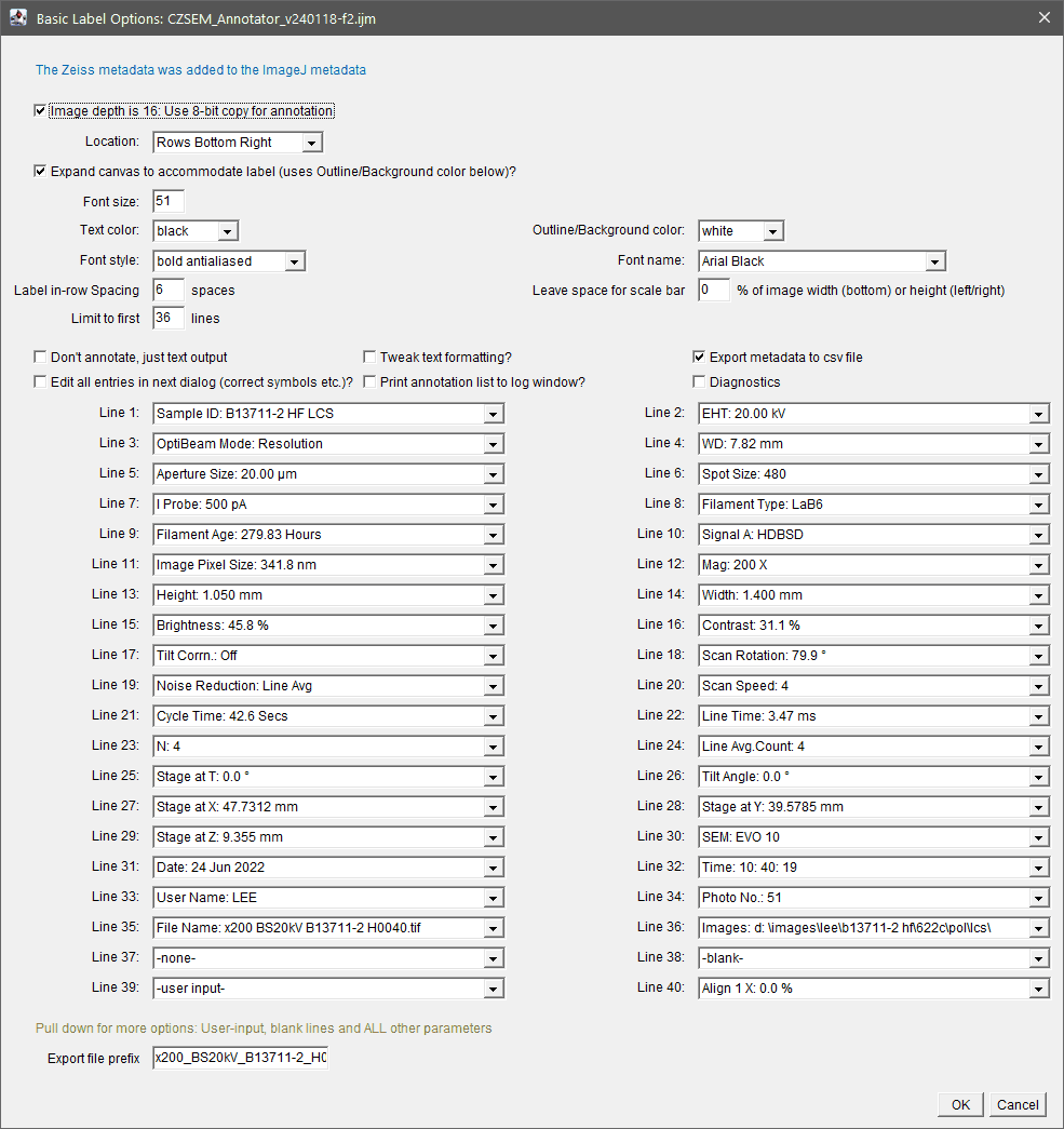
Carl Zeiss SmartSEM Metadata Utilities
These ImageJ macros use a variety of techniques to extract the metadata from SmartSEM images (link), the CZSEM_Metadata_To_Info and CZSEM_Transfer_MetadataToOtherImage macros use the tiff_tags plugin written by Joachim Wesner to extract the data.
The annotator macro (illustrated above) allows you to overlay up to 40 operating parameters onto a copy of the image (it will also automatically add the operating parameters to the ImageJ info header so that the copy will retain this information). Alternatively you can expand the canvas to display the annotation outside the image. The main menu can be seen below. The macro can be easily modified to create a custom annotation bar containing your favorite parameters. The annotation list can include blank lines and user input. The available formats and optional colors are the same as the "fancy labeling" macros.
The metadata-to-info macro will simply copy the embedded metadata to the ImageJ info header, allowing it to be saved with the image. The metadata-to-otherimage macro will copy the metadata to any other open image you select. The export macro will export the microscope parameters to a csv file in the same directory as the original image.
Return to Macro Collections menu
Set standard size selection or trimmed selections
This ImageJ/Fiji macro (link) allows you to make standard size or aspect selections or make selections that are trimmed full-image selections, trimmed to non-background features (binary images only) or trimmed selections. The resulting selection may be saved in the original image directory and reloaded for later reuse. The selection may also be added to the ROI manager and as an overlay. The selected setttings are stored in user preferences and become the default values for the next run. Using this macro makes it much easier to select image details of consistent sizes and shapes.
Return to Macro Collections menu
LUTs
Color lookup tables (LUTs) that are friendly to color-blind viewers and that are also easily converted to linear gradients for black and white printing in some journals can be useful. To this end we have modified the new "Viridis" LUT by Nathaniel Smith and Stéfan van der Walt so that it has a more linear conversion to gray:

We have also created a close-to-gray (a hint of blue) silver LUT that contrasts well with both gray and color images and converts well to non-color printing.

Both ASC LUTs are available from github. All the ASC macros assume that these LUTs are installed and places them as the primary selections.
Dichromacy can be simulated using Gabriel Landini's Dichromacy Plugin at this: link.
Return to Macro Collections menu
Notepad++ (NPP) Language Files
The free source code editor Notepad++ for Windows OS has some useful features for editing macros and it is easy to develop language files for specific applications such as ImageJ. Our language file for ImageJ/Fiji macros can be found in this repository along with the macro lists imported to make it.
IJMacro_Lang.xml is a "User Defined Language" (UDL) file for highlighting macro functions when editing macro scripts in Notepad++. For the current version of Notepad++ (for Windows) User Defined Language (UDL) files in xml format are placed in:
%AppData%\Roaming\Notepad++\userDefineLangs
The corresponding AutoComplete file (which also contains function usage information that will be dispayed in a pop-up window) is placed in the autoCompletion subfolder of the installation directory. This file must be given the same name as defined in the UDL file line:
<UserLang name="IJMacro" ext="ijm", udlVersion="2.1">
In the case above the autoCompletion file should be renamed "IJMacro.xml".
The usefulness of Notepad++ for coding ImageJ macro files can be greatly enhanced using the wide variety of available plugins. However, the implementation of auto code completion in the built-in imageJ/Fiji macro editor by Robert Haase in 2018 has been transformative in the usefulness of the built-in editor for learning the macro language. Patrice Mascalchi has also written an autocomplete file for Notepad++.
A useful feature of editing a macro in NPP is that using the NPP export plugin allows you to export syntax highlighted code to html or rtf (for use in word process). RTF copied into the clipboard can be directly pated into Word. The simple code below was exported from NPP NPP_ExportPlugin:
/* Very simple auto white balance using the ImageJ Bleach-correction plugin made available by Kota Miura and Jens Rietdorf (full plugin documentation available at https://wiki.cmci.info/downloads/bleach_corrector). v180710 first version of macro PJL NHMFL FSU */ setBatchMode(true); originalImage = getTitle(); run("Duplicate...", "title=temp"); run("RGB Stack"); run("Bleach Correction", "correction=[Simple Ratio] background=0"); run("Stack to RGB"); closeImageByTitle("DUP_temp"); closeImageByTitle("temp"); selectWindow("DUP_temp (RGB)"); rename(originalImage + "_awb"); setBatchMode("exit and display"); run("Collect Garbage"); showStatus("Auto White Balance Macro Completed"); /* Functions */ function closeImageByTitle(windowTitle) { /* Cannot be used with tables */ if (isOpen(windowTitle)) { selectWindow(windowTitle); close(); }Return to Macro Collections menu
The National High Magnetic Field Laboratory is supported by the National Science Foundation Division of Materials Research and the State of Florida. The Applied Superconductivity Center receives additional funding from the US Department of Energy, CERN and NIH.
This work is licensed under a Creative Commons Attribution 4.0 International License.Software is licensed under MIT license.